Fun finding duplicate elements in an array

I recently saw a fun programming challenge of trying to find a duplicate element in an array. The problem was stated as follows.

  • You have an integer array of length n.
  • Each element in the array can only take on the values of [0, n-1].
  • Try to find all integer values that are duplicated in the array.

For example, the array has a length of 5, thus containing only the values in the set {0, 1, 2, 3, 4} or range [0, 4] (note inclusive both ends). The actual array might hold elements (or integers) in this order: 2, 1, 4, 1, 3.

This problem is so silly to me, but it does have its merits, such as flushing out one’s understanding of worst case running time and space complexity. Before we begin, let’s list the approaches and their associated complexities. In the following table, the different solutions are given a name, followed by their running time and space complexity in big-Oh notation, and they are sorted by running time complexity descendingly and then space complexity descendingly.

name running time complexity space complexity
naive O(n^2) O(C)
sorting O(n log n) O(C)
map O(n) O(n)
set O(n) O(n)
bitmap O(n) O(n)
awesome O(n) O(C)

Continue reading

Running a cluster of virtual machines with Hadoop (HDFS + YARN) v2.4.1 and Spark v1.0.1 using Vagrant

I was able to set up a cluster of virtual machines (VMs) running Hadoop v2.4.1 with HDFS and YARN as well as Spark v1.0.1. The cluster setup was possible using Vagrant v1.5.1 and VirtualBox v4.3.10. The project is open source using Apache v2.0 License and is available at GitHub. I created this project for multiple reasons.

  • to learn about creating a cluster of VMs with Vagrant,
  • to have a sandbox with Hadoop (HDFS + YARN),
  • to have a sandbox with Spark, and
  • to AVOID having to download the sandbox VMs from Cloudera and Hortonworks (it takes forever to download these VMs; I, myself, was ever only able to finish downloading the CDH sandbox once, and yet, after 24+ hours, the file was corrupted; morever, these VMs are are standalone VMs and do not emulate the cluster environment).

To use this project you will need to install Vagrant and VirtualBox. You will also need to install a git client to clone the project from GitHub. After you have the above installed, then you can change into the cloned directory and simply type in

vagrant up

Continue reading

Bayesian scoring function Java and JavaScript API for Bayesian Belief Networks

The Bayesian Dirichlet (BD) scoring function is defined as follows.
P(B_S,D) = \prod_{i=1}^{n} \prod_{j=1}^{q_i} \left( \frac{\Gamma(N_{ij}^{'})}{\Gamma(N_{ij}^{'} + N_{ij})} \prod_{k=1}^{r_i} \frac{\Gamma(N_{ijk}^{'} + N_{ijk})}{\Gamma(N_{ijk}^{'})} \right)

Click this link to see what each of these terms mean.

For a weekend project, I created a Java and JavaScript API for computing the BD scoring function. The project is open-source with Apache License v2.0. You may download the project from GitHub at https://github.com/vangj/multdir-core.

Let’s see how we may quickly use these APIs to compute the score of a Bayesian Belief Network (BBN). In [Cooper92], a set of data with three variables (X1, X2, X3) was given as follows.

X1 X2 X3
p a a
p p p
a a p
p p p
a a a
a p p
p p p
a a a
p p p
a a a

There was also 3 Bayesian network structures (BS) to represent the relationships of the variables as well. Those 3 BS were reported as follows.

  • BS1: X1 → X2 → X3
  • BS2: X2 ← X1 → X3
  • BS3: X1 ← X2 ← X3

In Java, we can use the API to quickly estimate the scores of BS1, BS2, and BS3 as follows.

double bs1 = (new BayesianDirchletBuilder())
		.addKutato(5, 5) //X1
		.addKutato(1, 4) //X2
		.addKutato(4, 1)
		.addKutato(0, 5) //X3
		.addKutato(4, 1)
		.build()
		.get();
double bs2 = (new BayesianDirchletBuilder())
		.addKutato(5, 5) //X1
		.addKutato(1, 4) //X2
		.addKutato(4, 1)
		.addKutato(2, 3) //X3
		.addKutato(4, 1)
		.build()
		.get();
double bs3 = (new BayesianDirchletBuilder())
		.addKutato(1, 4) //X1
		.addKutato(4, 1)
		.addKutato(0, 4) //X2
		.addKutato(5, 1)
		.addKutato(6, 4) //X3
		.build()
		.get();

Likewise, in JavaScript, we can also quickly estimate the scores of these BBNs as follows.

var bs1 = (new BayesianDirichletBuilder())
	.addKutato([5,5])
	.addKutato([1,4])
	.addKutato([4,1])
	.addKutato([0,5])
	.addKutato([4,1])
	.build()
	.get();
var bs2 = (new BayesianDirichletBuilder())
	.addKutato([5,5])
	.addKutato([1,4])
	.addKutato([4,1])
	.addKutato([2,3])
	.addKutato([4,1])
	.build()
	.get();
var bs3 = (new BayesianDirichletBuilder())
	.addKutato([1,4])
	.addKutato([4,1])
	.addKutato([0,4])
	.addKutato([5,1])
	.addKutato([6,4])
	.build()
	.get();

Notice how in both APIs, you only add the counts? Easy.

Also, a working demo of using the JavaScript API to compute the BBN scores is in the repository for this project. Here’s a screenshot. Note that the scores are in log-space. Computing the score using factorials is not practical. In log-space, the lower the score associated with a BBN, the better the BBN.
multidir-ss

As always, enjoy and cheers! Sib ntsib dua nawb mog!

References

  • [Cooper92] G.F. Cooper and E. Herskovits. A Bayesian method for the induction of probabilistic networks from data. Machine Learning, 9, 309–347 (1992).

Installing a single-node Hadoop (v2.3.0) instance with YARN using Vagrant

In this blog, I will show how to install a single-node Hadoop (v2.3.0) instance with YARN using Vagrant. You might think this is a crazy idea, given that HortonWorks and Cloudera offers free sandboxes with Hadoop. However, it’s not so crazy if you think about wanting to learn about how to actually do it yourself (DIY). There’s a lot that one can learn with a DIY approach (such as dependencies and minimal requirements). Also, I find these sandboxes quite confusing (where’s Hadoop actually installed; you might find files are all over the place) and resembles bloatware (Spark, Hue, Impala, etc…). Furthermore, I found the installation documentation on Hadoop unclear, and I just had to figure out for myself what’s involved. To follow along in this blog, you will need to download the following software.

The first thing you need to do is install VirtualBox. The second thing you need to do is install Vagrant. Next, on the command-line, add the required Vagrant box.

vagrant box add centos65 https://github.com/2creatives/vagrant-centos/releases/download/v6.5.1/centos65-x86_64-20131205.box

Then, using your favorite Git client, check out the Vagrant project from GitHub at https://github.com/vangj/vagrant-hadoop-2.3.0.git. After you checkout the Vagrant project, go into this directory and simply type in the following.

vagrant up

Depending on your connection, it will take a while for the virtual machine (VM) to get created. The primary reason for the installation time is that after the VM is created, we have to download and install OpenJDK and Hadoop. The download of OpenJDK happens through using yum, while the download of Hadoop happens through the use of curl. The secondary reason is that I couldn’t store the Hadoop archive on GitHub (GitHub does not allow files larger than 50 MB), so, the workaround is to have Vagrant execute a script to download Hadoop.

After the VM finishes being created, you can SSH into the VM by typing the following.

vagrant ssh

When you are done with the VM, you can destroy it by using the following command.

vagrant destroy

But, before you destroy the VM, you may verify that Hadoop was successfully installed by pointing your browsers to the following URLs.

Note that the URLs are pointing to localhost and NOT the VM. The reason why this is possible is because Vagrant can setup port forwarding from your desktop to the VM. This feature is another reason why Vagrant is an awesome product.

You should also try the hdfs shell command.

hdfs dfs -ls /

Well, that is it for this blog. I hope and expect that we all can easily and at-will now setup our own sandboxes of Hadoop with YARN using Vagrant and VirtualBox. Now, we can move onto real fun things like building applications to run on YARN.

As always, cheers!

Visualizing RSVP data from the Data Science DC Meetup group

Recently, the Data Science DC Meetup group held a competition for their members to visualize their RSVP data. I did not have too much time, but I took a stab at trying to visualize the data. In one approach, I simply clustered the Meetup event titles into 4 groups using the k-means algorithm, and from each group/cluster, I created word clouds. In another approach, I built a n-by-n co-occurrence matrix, where n is the number of members and each matrix cell value was the number of times the i-th and j-th members went to the same Meetup event. From this matrix, I built a maximum weight spanning tree (MWST) where each vertex corresponded to a member and each edge was weighted by the co-occurrence value. I then visualized this MWST using the Yifu Han layout algorithm. The original data and visualizations may be downloaded below. 

  1. Original data.
  2. Word cloud visualization.
  3. Social network visualization.

As usual, cheers! Sib ntsib dua mog!

Constructing a ROC curve to measure and visualize the performace of a binary classifier

A very short blog post this time. I wrote a paper on how ROC curves are constructed to measure and visualize the performance of binary classifiers. If you are interested, you may download the paper by clicking here.

Enjoy and cheers! Sib ntsib dua nawb mog.إلى اللقاء

Bayesian scoring functions for structure learning of Bayesian belief networks (BBNs)

In this blog post, I’m going to be referring to a paper that I wrote about some Bayesian scoring functions for learning the structure of Bayesian belief networks (BBNs). The paper may be downloaded by clicking here, and there is also an accompanying slide deck that may be downloaded by clicking here. These documents are licensed under a Creative Commons Attribution 3.0 Unported License.

Define the following.

  • \textbf{X}=\{X_1,\ldots,X_n\} is a set of discrete random variables
  • \pi_i is the set of parents of X_i and \pi=\{\pi_1,\ldots,\pi_n\}
  • q_i 
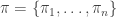
is the number of unique instantiations (configurations) of \pi_i
  • r_i is the number of values for X_i
  • N_{ijk} is the number of times (frequency of when) X_i=k and pi_i=j, and N_{ij} = \sum_k N_{ijk}
  • N_{ijk}^{'} 
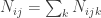
is the hyperparameter for when X_i=k and pi_i=j, and N_{ij}^{'} = \sum_k N_{ijk}^{'}
  • x!=\prod_{k=1}^{x} k is the factorial function
  • \Gamma(x) = (x-1)! 
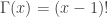
is the gamma function
  • B_S is the BBN structure
  • D is the data
  • P(B_S,D) is the joint probability of the BBN structure and data

Then, the Bayesian Dirichlet (BD) scoring function is defined as follows.
P(B_S,D) = \prod_{i=1}^{n} \prod_{j=1}^{q_i} \left( \frac{\Gamma(N_{ij}^{'})}{\Gamma(N_{ij}^{'} + N_{ij})} \prod_{k=1}^{r_i} \frac{\Gamma(N_{ijk}^{'} + N_{ijk})}{\Gamma(N_{ijk}^{'})} \right)

A few Bayesian scoring functions are variations of the BD scoring function. In particular, the Kutato (K2), Bayesian Dirichlet equivalence (BDe), and Bayesian Dirichlet equivalence uniform (BDeu) scoring functions are variants (special cases) of BD, and they differ in how they set the values of the hyperparameters. If you have ever wondered how these scoring functions (BD, K2, BDe, BDeu) were derived, the documents I wrote might give you some insight. In particular, I show how these scoring functions are based (in a sequential progression) on some basic mathematical functions (factorial, gamma, Beta), probability distributions (multinomial, Dirichlet, Dirichlet-multinomial), Bayes’ Theorem, and assumptions.

At any rate, happy reading! Sib nstib dua thiab thov kom muaj kev zoo siab rau koj xyoo tshiab no nawb mog!

Implementing RawComparator will speed up your Hadoop Map/Reduce (MR) Jobs

Introduction

Implementing the org.apache.hadoop.io.RawComparator interface will definitely help speed up your Map/Reduce (MR) Jobs. As you may recall, a MR Job is composed of receiving and sending key-value pairs. The process looks like the following.

  • (K1,V1) –> Map –> (K2,V2)
  • (K2,List[V2]) –> Reduce –> (K3,V3)

The key-value pairs (K2,V2) are called the intermediary key-value pairs. They are passed from the mapper to the reducer. Before these intermediary key-value pairs reach the reducer, a shuffle and sort step is performed. The shuffle is the assignment of the intermediary keys (K2) to reducers and the sort is the sorting of these keys. In this blog, by implementing the RawComparator to compare the intermediary keys, this extra effort will greatly improve sorting. Sorting is improved because the RawComparator will compare the keys by byte. If we did not use RawComparator, the intermediary keys would have to be completely deserialized to perform a comparison.
Continue reading

Controlling logging on Amazon Web Service’s (AWS) Elastic MapReduce (EMR) on a multi-node cluster

Introduction

Last time, I talked about controlling logging on Amazon Web Service’s (AWS) Elastic MapReduce (EMR). However, that approach works only when you provision an EMR cluster of 1 node and need to get the log files from that 1 node. In this blog, I will talk about how to control logging for an EMR cluster of more than 1 node. In fact, you should probably read the original article before reading this one because the approach is identical except for that the way you pull/acquire your custom log files is different.
Continue reading

An approach to controlling logging on Amazon Web Services’ (AWS) Elastic MapReduce (EMR)

Intro

I have been using the Elastic MapReduce (EMR) product. EMR is one of many products and services available from Amazon Web Services (AWS). EMR is AWS’s product to dynamically provision a Hadoop cluster. One problem I ran into was how to control logging. Hadoop uses Apache Commons Logging. Both Hadoop and AWS seem to encourage using Log4j as the actual logging implementation. This blog assumes you are familiar with all these components.

One problem I ran into was how to control logging using Apache Commons Logging and Log4j. What I wanted to do was to simply be able to specify logging properties for Log4j. I asked for help on the AWS EMR discussion forum, but for several days (and thus far), no one responded (where did all the AWS/EMR evangelists go?). From digging around the AWS site and other discussion threads, I did get some scattered “hints” of how to go about controlling logging. Still, when I searched for a more detailed explanation (on the general internet) putting all the parts together, I did not see anything helpful or instructive. But, with some perseverance, I did pull through and found a way, reported in this blog, to control logging on an AWS EMR Hadoop cluster.

As you may already know, there is a conf directory inside the root of the Hadoop installation directory (i.e. /home/hadoop/conf). Inside this directory, is a log4j.properties file (i.e. /home/hadoop/conf/log4j.properties). This file is precisely where you need to make modifications to control logging.
Continue reading